The new visual identity of my work place (and the re-ignition of an old lava lamp) made me think of the good old metaballs from the Amiga demo-scene of yonder and how it has been a while since I have implemented them from scratch. This time I wanted to play around with Python and numpy to see what that could bring.
But first, what are metaballs?
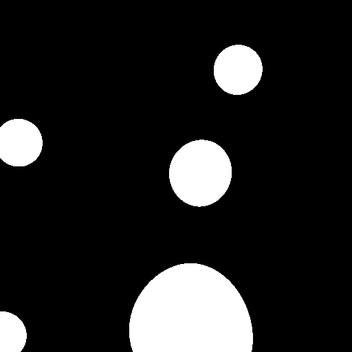
It’s, for example, this:
Wikipedia defines them as:
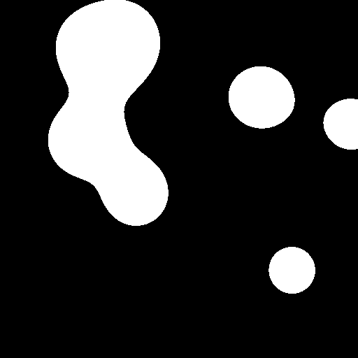
In computer graphics, metaballs are organic-looking n-dimensional isosurfaces, characterised by their ability to meld together when in close proximity to create single, contiguous objects. https://en.wikipedia.org/wiki/Metaballs
As cool as multidimensional metaballs are, we’ll stick to 2D ones in this post.
The algorithm
The algorithm behind them is quite straightforward – in their simplest form. Basically for each pixel in each frame, or buffer, you add up the influence of each metaball in the simulation and then cut off below a certain threshold and normalize what’s left. The influence function can be a simple “ball-power” over euclidean distance calculation.
So, for each pixel you get:
def generate_buffer_raw(buff, balls):
    for x in range(0, buff.shape[0]):
        for y in range(0, buff.shape[1]):
            for b in balls:
                d = dist([x,y], b.pos)
                if d == 0:
                    d = 1 # not correct, per se, but, alas, it works...
                effect = b.rad / d
                buff[x,y] += effect
    return buff
And then you can apply the threshold, like so:
def apply_threshold(buff,threshold, margin=0):
    s1 = buff < (threshold - margin)
    s2 = buff > (threshold + margin)
    buff[:] = 255
    buff[s1] = 0
    if margin>0:
        buff[s2] = 0
    return buff
(With this threshold function we can also generate membrane style metaballs, but more on that later.)
First go: Pythagoras
My first go at this was just a brute force by using Pythagoras to calculate the euclidean distance.
def dist_sqrt(p1,p2):
    return math.sqrt((p1[0]-p2[0])**2 + (p1[1]-p2[1])**2)
The main loop is then just:
images = []
for _ in range(0, FRAMES):
    buff = generate_buffer(np.zeros((WIDTH, HEIGHT)), balls)
    buff = apply_threshold(buff, THRESHOLD, MARGIN)
    im = img.fromarray(buff).convert("RGB")
    images.append(im)
    update_balls(balls)
Where update_balls is simply a updating the position of the metaballs given their velocity — bouncing on the “walls” of our simulation, but, importantly not other balls.
And lo and behold there were metaballs.

However, as expected, this was rather slow. 100 frames of 128 by 128 clocking in at 46.5s on my macbook air from 2013.
46.5 s ± 0 ns per loop (mean ± std. dev. of 1 run, 1 loop each)
(For fun I ran the same code using Juno on my phone, and runtime went down to about 17s!)
As you might have guessed the costly computation is the distance function, so I went about experimenting.
Take two: numpy.linalg.norm
By naively replacing the distance function from with the equivalent linear algebra norm, we get:
def dist_linalg(p1,p2):
    return np.linalg.norm(p1 - p2)
This led to the same metaballs, but, alas, a higher runtime of 2min 47s!
Take three: precalculations
Next attempt to investigate precalculation of the computationally costly square root function needed in my first approach.
sqrt_precalc = {}

for i in np.arange(0, WIDTH ** 2 + HEIGHT ** 2):
    sqrt_precalc[int(i)] = math.sqrt(i)

def dist_precalc(p1,p2):
    i = (p1[0] - p2[0]) ** 2 + (p1[1] - p2[1]) ** 2
    return sqrt_precalc[int(i)]
This did shave off some seconds, and runtime went down to 42s.
Yet another approach: moar precalc!
I left it at that, thinking that the future of this would be to look into cheaper distance approximations to cut away parts of the buffer where no metaball could show up, but in my sleep another solution appeared… I was thinking that one could go further with the precalculations and precalculate “fields” of influence for each ball, or “radius”, and use proper linear algebra to get rid of some for loops.
def precalculate_field(ball, dim):
    buff = np.zeros(dim*2)
    ball = Ball([WIDTH, HEIGHT],ball.rad,np.array([0,0]))
    return generate_buffer_raw(buff, [ball])

fields = {}
for b in balls:
    if int(b.rad) not in fields.keys():
        fields[int(b.rad)] = precalculate_field(b, np.array([WIDTH, HEIGHT]))
As you can see, to accommodate all possible positions of the balls I generate a field of influence that is 4 times larger than the output buffer.
Then I updated the generate buffer function to look like this:
def generate_buffer_precalc(buff, balls):
    for b in balls:
        x1 = WIDTH - int(b.pos[0])
        y1 = HEIGHT - int(b.pos[1])
        field = fields[int(b.rad)]
        window = field[x1:x1+WIDTH,y1:y1+HEIGHT]
        buff += window
    return buff
The main trick here is to move the field in place so that it covers the buffer based on where the ball in question is – a window into it, if you want. The only for loop now is over the balls themselves, and a simple linear algebra addition operation suffices to generate the resulting buffer of accumulated influence.
And lo and behold it was fast! A thousand fold increase over the best approach so far!
40 ms ± 687 µs per loop (mean ± std. dev. of 7 runs, 10 loops each)
Admittedly it consumes more memory, but hey, memory is cheap, time is money.
Some caveats:
- It is slightly less precise since it doesn’t do decimal places. (Yet!) (You still get good-enough-looking metaballs, methinks.)
- The precalulculation of the “fields” are not taken into account when reporting the run-time, but that is surprisingly fast – and only done once per “radius” of metaball…
More importantly, like this I can implement a real time version of this at some point using, let’s say pygame.
Ah, yes, I promised membranes, here’s a gif: